Snake Detection Hypothesis - Neural Net Foundations

Neural Net Foundations

---

---

Background

A study by Nagoya University on the Snake Detection Hypothesis suggests that human vision is tuned to more easily detect a potential danger, snakes. By obscuring images completely and taking incremented steps (5% correction to baseline), they were able to gauge differences in how obscured an image could remain while being identified.

As I’m studying neural nets, I thought as an interesting project I could replicate the study using a computer vision (CV) model. Assuming the hypothesis is true and human vision is evolutionarily tuned to more readily detect snakes, then the correlation should not be seen when tested by a CV model. Assuming that is the result, this may suggest that features specific to snakes do not make them more easily recognizable. Snakes do have a distinctive body type when compared to most other animals, including the animals used in the study.

The study used snakes, birds, cats and fish. The dataset is not publicly available, but there are fortunately plenty of publicly available models suited for the project. I have chosen ImageNet, since it is a large and well known dataset.

This initial NN is based off of fastai’s imagenette, which is designed to be small and capable for quick training and evaluation at the early stages of the development process. With only 10 classes, each distinct from each other, you can get a workable and performant model.

Let’s start with our imports, load our data and targets, and a few custom functions to keep things clean:

from fastai.vision.all import *
path = Path('/Users/ossie/sdhnet/data/animals/imagenette2-160/')

lbl_dict = dict(
    n01440764='tench',
    n02102040='English springer',
    n02979186='cassette player',
    n03000684='chain saw',
    n03028079='church',
    n03394916='French horn',
    n03417042='garbage truck',
    n03425413='gas pump',
    n03445777='golf ball',
    n03888257='parachute',
    birds='bird'
)

def label_func(fname):
  return lbl_dict[parent_label(fname)]

def get_lr(learn):
    lr_min, lr_steep = learn.lr_find(suggest_funcs=(minimum, steep))
    res = round( ( (lr_min + lr_steep)/2 ), 5)
    print('Learning rate finder result: ', res)
    return res

Datablocks & Batches

---

---

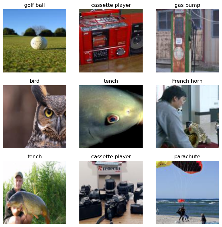
As part of the development process, it is encouraged to check that everything works in each step. Let’s check a batch from our DataBlock:

dblock = DataBlock(blocks = (ImageBlock, CategoryBlock),
                   get_items = get_image_files,
                   get_y = label_func,
                   splitter = GrandparentSplitter(),
                   item_tfms = RandomResizedCrop(128, min_scale=0.35),
                   batch_tfms = Normalize.from_stats(*imagenet_stats))
dls = dblock.dataloaders(path, batch_size=64)
dls.show_batch()

Experimenting with different batch sizes, 64 is working well for the size of the dataset (700 - 900 images per category). There was some, but minimal drop in performance at smaller batch sizes of 32. Using a larger batch size can potentially increase performance by reducing training time, which is a high priority goal when producing your MVP.

---

---

I’ve run into a few issues where I had a training set, but no valid set created. Let’s make sure we’ve got both in our DataLoaders:

dls.train_ds

(#10237) [(PILImage mode=RGB size=231x160, TensorCategory(1)),(PILImage mode=RGB size=240x160, TensorCategory(1)),(PILImage mode=RGB size=213x160, TensorCategory(1)),(PILImage mode=RGB size=228x160, TensorCategory(1)),(PILImage mode=RGB size=160x236, TensorCategory(1)),(PILImage mode=RGB size=213x160, TensorCategory(1)),(PILImage mode=RGB size=160x240, TensorCategory(1)),(PILImage mode=RGB size=213x160, TensorCategory(1)),(PILImage mode=RGB size=210x160, TensorCategory(1)),(PILImage mode=RGB size=160x236, TensorCategory(1))…]

---

---

dls.valid_ds

(#4117) [(PILImage mode=RGB size=213x160, TensorCategory(1)),(PILImage mode=RGB size=239x160, TensorCategory(1)),(PILImage mode=RGB size=160x200, TensorCategory(1)),(PILImage mode=RGB size=240x160, TensorCategory(1)),(PILImage mode=RGB size=240x160, TensorCategory(1)),(PILImage mode=RGB size=160x225, TensorCategory(1)),(PILImage mode=RGB size=235x160, TensorCategory(1)),(PILImage mode=RGB size=160x160, TensorCategory(1)),(PILImage mode=RGB size=160x225, TensorCategory(1)),(PILImage mode=RGB size=160x213, TensorCategory(1))…]

---

---

Learners, Metrics and Training

With that in check, it’s time to create our learner. For the metrics, I’ve chosen accuracy, in addition to F1 Score which is a combination of ‘precision’ and ‘recall’. The F1 score should give us an understanding of how accurately positive or true predictions were correct (precision), and of all the potential positive instances, how many were identified (recall) as single, balanced, metric. By setting the average='micro', we will be able to see one score with each individual class weighed equally.

We won’t be using a pre-trained model, as I’m looking to create a simple model with not too many features or attributes already trained into the network. The end goal is to compare the study with three to four CV models, with varying levels of training. Since this is the prototype and we want it quick to achieve a MVP, we can train on ResNet18. This is the smallest of the of the standard ResNet models, and should train the fastest. It should be easy to scale to a deeper network with more layers as the project progresses.

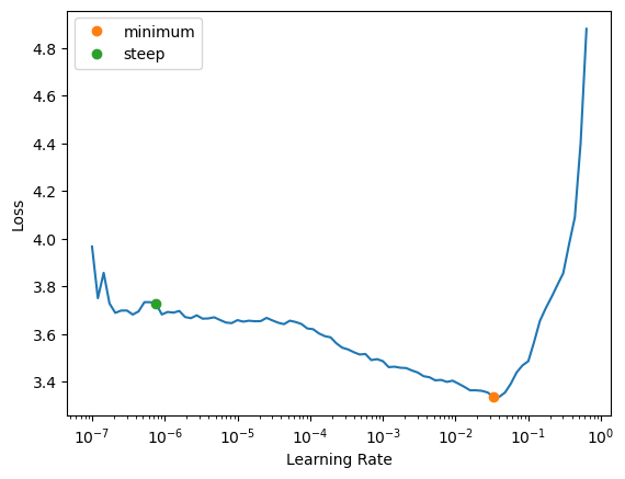
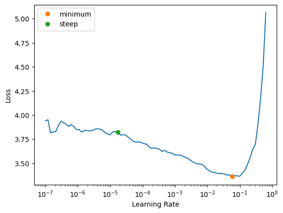
It’s important to also tune the learning rate. My custom function here is leveraging fast.ai’s lr_find(), an example used here in the docs.

learn = vision_learner(dls, resnet18, metrics=[accuracy, F1Score(average='micro')], pretrained=False)
lr = get_lr(learn)

Learning rate finder result: 0.00166

Our learning rate is the midpoint between where the steepest decrease in loss occurs, and the minimum where our loss diverges and begins to increase. This should be a nice goldilocks zone that balances too low a learning rate (meaning many epochs needed to achieve a working model) and our learning rate being too large (accuracy does not reliably increase).

learn.fit_one_cycle(10, lr)

epoch	train_loss	valid_loss	accuracy	f1_score	time
0	1.423258	1.712628	0.478990	0.478990	00:39
1	1.623324	1.930002	0.407335	0.407335	00:38
2	1.597714	1.856789	0.448385	0.448385	00:38
3	1.467201	1.617843	0.532184	0.532184	00:37
4	1.352724	1.541756	0.515181	0.515181	00:38
5	1.218052	1.280943	0.580277	0.580277	00:38
6	1.048109	0.969238	0.684965	0.684965	00:38
7	0.921193	0.928279	0.698567	0.698567	00:38
8	0.832626	0.799489	0.748603	0.748603	00:37
9	0.779347	0.783034	0.746417	0.746417	00:38

---

---

interp = ClassificationInterpretation.from_learner(learn)
interp.plot_confusion_matrix(figsize=(10, 10))

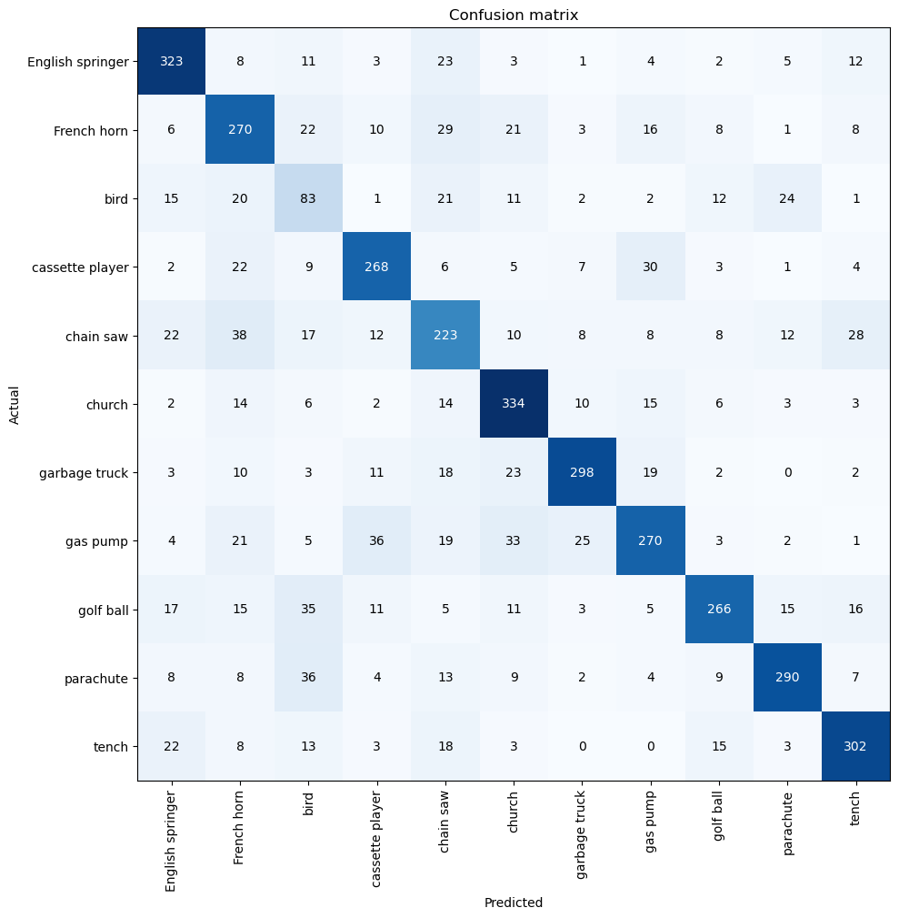
The accuracy on predicting birds isn’t bad, but not quite matching the perfomance of the other targets.

---

---

Matching the study’s data

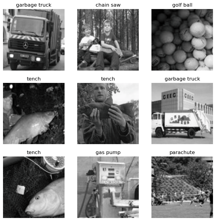
Unfortunately, the data set used for the study is not publicly available. I wasn’t able to gather specific examples of size, source or other methods of data collection and so I chose ImageNet as a standard data source. The discrepancy in performance between target categories may be due to data set size (it’s on the lower end of our range), but it should be constructive to first bring our existing data closer to the study conditions. The Nagoya study used grayscale images, so converting the images and measuring performance again should give more insight into how well our model performs for our task.

One simple change can convert our images to grayscale, using the Python Image Library (PIL) in our ImageBlock.

dblock = DataBlock(blocks = (ImageBlock(cls=PILImageBW), CategoryBlock),
                   get_items = get_image_files,
                   get_y = label_func,
                   splitter = GrandparentSplitter(),
                   item_tfms = RandomResizedCrop(128, min_scale=0.35),
                   batch_tfms = Normalize.from_stats(*imagenet_stats))

dls = dblock.dataloaders(path, batch_size=64)
dls.show_batch()

---

---

learn = vision_learner(dls, resnet18, metrics=[accuracy, F1Score(average='micro')], pretrained=False)
lr = get_lr(learn)
learn.fit_one_cycle(10, lr)

Learning rate finder result: 0.00289

epoch	train_loss	valid_loss	accuracy	f1_score	time
0	2.667787	2.205018	0.347583	0.347583	00:37
1	2.083144	17.378586	0.137722	0.137722	00:37
2	1.813329	1.876499	0.431868	0.431868	00:37
3	1.767364	2.764703	0.254311	0.254311	00:37
4	1.703397	2.122186	0.382074	0.382074	00:37
5	1.481549	1.390573	0.549672	0.549672	00:37
6	1.329995	1.245291	0.599951	0.599951	00:38
7	1.162172	1.026676	0.678164	0.678164	00:37
8	1.014946	0.946047	0.691037	0.691037	00:37
9	0.947772	0.897824	0.710955	0.710955	00:37

---

---

bw_metrics = learn.recorder.metrics
interp = ClassificationInterpretation.from_learner(learn)
interp.plot_confusion_matrix(figsize=(10, 10))

Comparing the two confusion matrices, it looks like removing color resulted in a significant decrease in accuracy for the birds category, with some slight loss on others. In particular, it looks like bird more frequently gets confused with parachute. I’d guess this is because these two can be seen in the same context or setting - flying - and color features of things like the sky stand out. However, correlations with things like ‘chain saw’ and ‘birds’ are less clear, so I will be doing some feature visualization down the line to better break down what’s happening here.